Getting started

Pymablock workflow

Getting started with Pymablock is simple, let’s start by importing it together with numpy.

import pymablock
import numpy as np

Let’s apply perturbation theory to a diagonal Hamiltonian with two subspaces \(A\) and \(B\), coupled by a perturbation.

1. Define a Hamiltonian

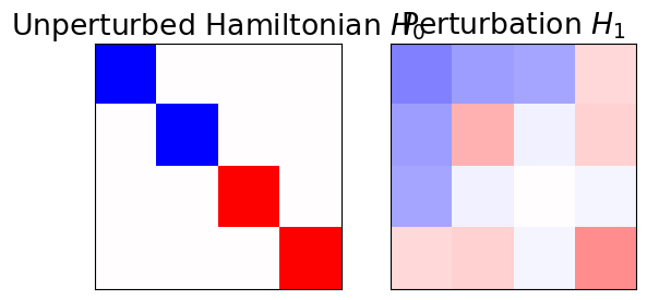
We begin by defining a Hamiltonian and a random perturbation.

# Diagonal unperturbed Hamiltonian
H_0 = np.diag([-1., -1., 1., 1.])

# Random Hermitian matrix as a perturbation
def random_hermitian(n):
    H = np.random.randn(n, n) + 1j * np.random.randn(n, n)
    H += H.conj().T
    return H

H_1 = 0.2 * random_hermitian(4)

While \(H_0\) has two subspaces separated in energy, \(H_1\) couples them.

Show code cell source Hide code cell source

import matplotlib.pyplot as plt

fig, (ax_0, ax_1) = plt.subplots(ncols=2)

ax_0.imshow(H_0.real, cmap='seismic', vmin=-2, vmax=2)
ax_0.set_title(r'Unperturbed Hamiltonian $H_0$')
ax_0.set_xticks([])
ax_0.set_yticks([])

ax_1.imshow(H_1.real, cmap='seismic', vmin=-2, vmax=2)
ax_1.set_title(r'Perturbation $H_1$')
ax_1.set_xticks([])
ax_1.set_yticks([]);

Subspaces must be separated

For the perturbation theory to work, the spectra of the two subspaces must differ. The larger the smallest energy difference between the two subspaces, the better the perturbation theory works.

2. Define the perturbative series

Most Pymablock users will need only one function: block_diagonalize. It takes all the possible types of input and defines a solution of the perturbation theory problem as infinite series of the transformed Hamiltonian \(\tilde{H}\) and the corresponding transformation \(U\).

from pymablock import block_diagonalize

hamiltonian = [H_0, H_1]

H_tilde, U, U_adjoint = block_diagonalize(hamiltonian, subspace_indices=[0, 0, 1, 1])

Here the first term in the hamiltonian list is the unperturbed Hamiltonian \(H_0\), and the following terms are the perturbations. The subspace_indices argument defines to which subspace each diagonal term of \(H_0\) belongs.

This does do any computations yet, and only defines the answer as an object that we can query.

Most users will only ever need the diagonal blocks of H_tilde, however Pymablock returns the extra information in case it is needed.

3. Get the perturbative results

To get perturbative corrections to the diagonal blocks of the Hamiltonian, we query H_tilde with the block and the order of the correction.

For example, we obtain a second order correction to the first subspace as

H_tilde[0, 0, 2]

array([[-0.13106371+0.j        ,  0.06659443-0.05802661j],
       [ 0.06659443+0.05802661j, -0.16023586+0.j        ]])

where (0, 0) is the first subspace (\(AA\) block), and 2 means the second order correction.

Let us also check that the off-diagonal blocks of the Hamiltonian are \(0\) to any order.

H_tilde[0, 1, 3]

zero

What does zero mean?

Some terms in series are completely missing. Because Pymablock supports very different types of operators, it is impossible to have a single one-size-fits-all value for a zero element. Therefore Pymablock implements its own sentinel values to represent zero and one. These special values also help the library’s performance by allowing for to skip unnecessary computations. Typically, they should not appear in user code, however you may encounter them in rare cases. You can then use expressions like if result is pymablock.series.zero to check for their occurrence and handle them.

where (0, 1) is the \(AB\) block, and 3 is the third order correction.

Just like H_tilde, U and U_adjoint are BlockSeries objects too. In most situations these are not necessary, but they can be useful to transform any other observable to the basis of the H_tilde.

To get more than one perturbative correction at a time, we can query H_tilde using numpy’s indexing convention. For example, we query the corrected Hamiltonian of the first subspace up to second order using

H_tilde[0, 0, :3]

masked_array(data=[<Compressed Sparse Column sparse array of dtype 'float64'
                   	with 2 stored elements and shape (2, 2)>                ,
                   array([[-0.49811759+0.j        , -0.37901235-0.19517022j],
                          [-0.37901235+0.19517022j,  0.30732665+0.j        ]]),
                   array([[-0.13106371+0.j        ,  0.06659443-0.05802661j],
                          [ 0.06659443+0.05802661j, -0.16023586+0.j        ]])],
             mask=False,
       fill_value=np.str_('?'),
            dtype=object)

The output is a MaskedArray with the same block structure as if we queried a numpy array with the same indices. The entries of this array are the Hamiltonian terms themselves, and therefore they may be of different types: here we see that the unperturbed Hamiltonian is stored as a sparse matrix, while the higher orders are numpy arrays.

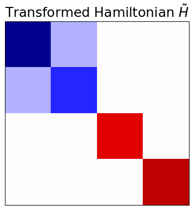
The final block-diagonalized Hamiltonian up to second order looks like this:

Show code cell source Hide code cell source

import numpy.ma as ma
from scipy.linalg import block_diag

transformed_H = ma.sum(H_tilde[:2, :2, :3], axis=2)
block = block_diag(transformed_H[0, 0], transformed_H[1, 1])

fix, ax_2 = plt.subplots()
ax_2.imshow(block.real, cmap='seismic', vmin=-2, vmax=2)
ax_2.set_title(r'Transformed Hamiltonian $\tilde{H}$')
ax_2.set_xticks([])
ax_2.set_yticks([]);

Masked arrays skip entries

NumPy’s masked arrays are arrays where some entries are masked out because they are undefined, or because they are not needed, such that they are skipped in various operations. In Pymablock, we use masked arrays to skip the terms that are zero, so that they are skipped in summation and multiplication throughout the algorithm. To sum over the entries of a masked array, use np.ma.sum(array), for example.

Further capabilities

Let us now consider a more complex example, where:

• The unperturbed Hamiltonian is not diagonal

• There are multiple perturbative parameters

• Some perturbations are not first order

• We want to separate the Hamiltonian into more than two subspaces

Because diagonalization is both standard, and not our focus, Pymablock will not do it for us. However, it will properly treat a non-diagonal unperturbed Hamiltonian if we provide its eigenvectors.

General Hamiltonians

Let’s define a problem with two perturbative parameters:

(1)\[\begin{equation} H = H_{00} + \lambda_1 H_{10} + \lambda_1^2 H_{20} + \lambda_2 H_{01} \end{equation}\]

H_00 = random_hermitian(7)  # Unperturbed Hamiltonian
H_10 = 0.1 * random_hermitian(7)  # Linear term in the first perturbative parameter
H_20 = 0.1 * random_hermitian(7)  # Quadratic term in the first perturbative parameter
H_01 = 0.1 * random_hermitian(7)  # Linear term in the second perturbative parameter
hamiltonian = {(0, 0): H_00, (1, 0): H_10, (2, 0): H_20, (0, 1): H_01}

The keys of the hamiltonian dictionary are tuples of integers, where \(i\)-th integer is the order of the \(i\)-th perturbative parameter.

Efficiency hint

The Hamiltonian does not contain values of \(\lambda_1\) and \(\lambda_2\). Instead, to evaluate \(\tilde{H}\), we will provide the values of the perturbative parameters at the last step.

If you want to vary the perturbation strength, providing its values last is more efficient than recomputing the perturbative series.

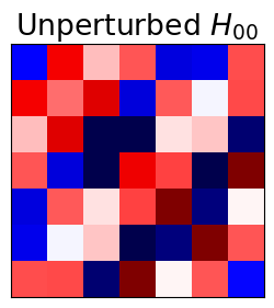
Differently from the first example, \(H_{00}\) is not diagonal anymore

Show code cell source Hide code cell source

plt.figure(figsize=(3, 3))
plt.imshow(H_00.real, cmap='seismic', vmin=-2, vmax=2)
plt.title(r'Unperturbed $H_{00}$')
plt.xticks([])
plt.yticks([]);

Specifying the subspaces

To define the perturbative series we compute the eigenvectors of \(H_{00}\) and split them into groups that define the different subspaces. In this case, we separate the Hamiltonian into three subspaces: \(A\), \(B\), and \(C\).

_, evecs = np.linalg.eigh(H_00)
subspace_eigenvectors = [evecs[:, :3], evecs[:, 3:6], evecs[:, 6:]]  # three subspaces

H_tilde, U, U_adjoint = block_diagonalize(
  hamiltonian=hamiltonian, subspace_eigenvectors=subspace_eigenvectors
)

Important

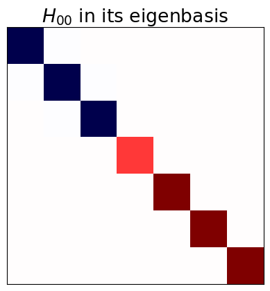
block_diagonalize transforms everything to the basis of subspace_vectors, such that, for example, the unperturbed Hamiltonian becomes diagonal.

Accordingly U is the unitary transformation that block-diagonalizes the Hamiltonian in the eigenbasis of \(H_0\).

Show code cell source Hide code cell source

from scipy.sparse import block_diag

H_0 = block_diag(H_tilde[[0, 1, 2], [0, 1, 2], 0, 0]).toarray()

fix, ax_2 = plt.subplots()
ax_2.imshow(H_0.real, cmap='seismic', vmin=-2, vmax=2)
ax_2.set_title(r'$H_{00}$ in its eigenbasis')
ax_2.set_xticks([])
ax_2.set_yticks([]);

Querying the perturbative series

Let us examine how the perturbative series is stored in H_tilde, which is a BlockSeries object.

It has a \(3\times 3\) block structure corresponding to the \(A\), \(B\), and \(C\) subspaces. The number of its infinite size dimensions is the number of perturbative parameters.

f"{H_tilde.shape=}, {H_tilde.n_infinite=}"

'H_tilde.shape=(3, 3), H_tilde.n_infinite=2'

BlockSeries defines a way to compute its entries, which are stored in the internal _data attribute. Before we did any computation, _data is empty

f"{H_tilde._data=}, {U._data=}"

'H_tilde._data={}, U._data={(0, 0, 0, 0): one, (1, 1, 0, 0): one, (2, 2, 0, 0): one}'

Querying a multivariate BlockSeries requires either specifying only the block indices, or blocks and orders of all its perturbations.

For example, here define a new BlockSeries that only contains the \(A\) and \(B\) subspaces

H_tilde_subblocks = H_tilde[:2, :2]
print(type(H_tilde_subblocks))
print(H_tilde_subblocks.shape)
print(H_tilde_subblocks.n_infinite)

<class 'pymablock.series.BlockSeries'>
(2, 2)
2

Alternatively, here we compute a term of \(\tilde{H}^{AA}\) of the order \(\lambda_1^2\lambda_2^3\)

%time H_tilde[0, 0, 2, 3]

CPU times: user 33.6 ms, sys: 915 μs, total: 34.5 ms
Wall time: 34.3 ms

array([[-2.81438676e-05+0.00000000e+00j,  7.67128562e-05+2.87940349e-05j,
        -7.03149114e-05+7.77958685e-07j],
       [ 7.67128562e-05-2.87940349e-05j, -3.75514465e-05+0.00000000e+00j,
         7.10040542e-05-2.69137510e-05j],
       [-7.03149114e-05-7.77958685e-07j,  7.10040542e-05+2.69137510e-05j,
        -2.71260814e-04+0.00000000e+00j]])

Computing this term required also computing several orders of U, which are now stored in U._data

f"{len(H_tilde._data.keys())=}, {len(U._data.keys())=}"

'len(H_tilde._data.keys())=1, len(U._data.keys())=3'

That means that querying the same term of \(\tilde{H}^{AA}\) is now nearly instantaneous

%time H_tilde[0, 0, 2, 3]

CPU times: user 43 μs, sys: 8 μs, total: 51 μs
Wall time: 52.9 μs

array([[-2.81438676e-05+0.00000000e+00j,  7.67128562e-05+2.87940349e-05j,
        -7.03149114e-05+7.77958685e-07j],
       [ 7.67128562e-05-2.87940349e-05j, -3.75514465e-05+0.00000000e+00j,
         7.10040542e-05-2.69137510e-05j],
       [-7.03149114e-05-7.77958685e-07j,  7.10040542e-05+2.69137510e-05j,
        -2.71260814e-04+0.00000000e+00j]])

The same is true for BlockSeries objects that were defined by slicing H_tilde

%time H_tilde_subblocks[0, 0, 2, 3]

CPU times: user 4.93 ms, sys: 0 ns, total: 4.93 ms
Wall time: 4.89 ms

array([[-2.81438676e-05+0.00000000e+00j,  7.67128562e-05+2.87940349e-05j,
        -7.03149114e-05+7.77958685e-07j],
       [ 7.67128562e-05-2.87940349e-05j, -3.75514465e-05+0.00000000e+00j,
         7.10040542e-05-2.69137510e-05j],
       [-7.03149114e-05-7.77958685e-07j,  7.10040542e-05+2.69137510e-05j,
        -2.71260814e-04+0.00000000e+00j]])

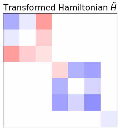
The final \(3 \times 3\) block-diagonalized Hamiltonian up to second order in each perturbative parameter looks like this:

Show code cell source Hide code cell source

import numpy.ma as ma
from scipy.linalg import block_diag

transformed_H = ma.sum(H_tilde[:3, :3, :2, :2], axis=(2, 3))
block = block_diag(transformed_H[0, 0], transformed_H[1, 1], transformed_H[2, 2])

fix, ax_2 = plt.subplots()
ax_2.imshow(block.real, cmap='seismic', vmin=-2, vmax=2)
ax_2.set_title(r'Transformed Hamiltonian $\tilde{H}$')
ax_2.set_xticks([])
ax_2.set_yticks([]);

Transforming other operators

Earlier we saw that Pymablock computes the Hamiltonian and the unitary transformation as ~pymablock.series.BlockSeries objects. While the Hamiltonian is the most important object, the unitary transformation allows to transform any other operator to the basis of the of the perturbed Hamiltonian. These operators may be density matrices, other Hamiltonians, or any other observable.

Here we create the unperturbed Hamiltonian H_0, the perturbation H_1, and an additional operator X that we want to transform to the basis of effective Hamiltonian. First, we perform the block diagonalization.

H_0 = random_hermitian(4)
H_1 = 0.1 * random_hermitian(4)
X = random_hermitian(4)
_, evecs = np.linalg.eigh(H_0)

H_tilde, U, U_adjoint = block_diagonalize(
    [H_0, H_1], subspace_eigenvectors=[evecs[:, :2], evecs[:, 2:]]
)

Because block_diagonalize parses the input Hamiltonian and separates it into blocks using subspace_indices or subspace_eigenvectors, we first need to convert X into a BlockSeries object in the same basis as H_0 and with the same perturbative parameters and block structure. We do this by using operator_to_BlockSeries function, which has inputs similar to block_diagonalize, and use the dictionary format to indicate that X depends on a single perturbative parameter.

X_series = pymablock.operator_to_BlockSeries(
    {(0,): X},
    name="X",
    hermitian=True,  # Not important here, but slightly improves performance.
    subspace_eigenvectors=[evecs[:, :2], evecs[:, 2:]]
)

Finally, to compute X in the perturbed basis, we multiply it by the unitary transformation.

X_tilde = pymablock.series.cauchy_dot_product(U_adjoint, X_series, U)

In zeroth order X and X_tilde coincide, but X_tilde contains the perturbative corrections. Let us confirm this, and check the second order correction to the projection of X on the \(A\) subspace.

assert np.allclose(X_tilde[0, 0, 0], X_series[0, 0, 0])
X_tilde[0, 0, 2]

array([[ 0.05676398-3.26296128e-19j, -0.06213413+9.53315274e-02j],
       [-0.06213413-9.53315274e-02j,  0.06825824+9.10864868e-19j]])

Selective diagonalization

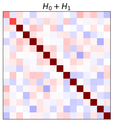
As an alternative to separating a Hamiltonian into blocks, Pymablock is capable of perturbatively canceling arbitrary off-diagonal terms in a Hamiltonian. The only requirement is that any two states to decouple are not degenerate, unless they are already decoupled. Let us illustrate this using a Hamiltonian \(H_0 + H_1\):

N = 16
H_0 = np.diag(np.arange(N) + 0.2 * np.random.randn(N))
H_1 = 0.1 * np.random.randn(N, N)
H_1 += H_1.T

plt.imshow(H_0 + H_1, cmap='seismic', vmin=-2, vmax=2)
plt.title(r'$H_0 + H_1$')
plt.xticks([])
plt.yticks([]);

We define a mask that selects the terms to keep in the Hamiltonian. To show the arbitrary nature of the mask, we use a smiley face.

smiley_binary = np.array(
    [
        [1, 1, 0, 0, 0, 1, 1],
        [1, 1, 0, 0, 0, 1, 1],
        [0, 0, 0, 1, 0, 0, 0],
        [0, 0, 0, 1, 0, 0, 0],
        [1, 0, 0, 0, 0, 0, 1],
        [0, 1, 1, 1, 1, 1, 0],
    ],
    dtype=bool,
)

mask = np.zeros((N, N), dtype=bool)
mask[1:smiley_binary.shape[0] + 1, -smiley_binary.shape[1] - 1:-1] = smiley_binary
mask = ~(mask | mask.T)
np.fill_diagonal(mask, False)

plt.imshow(mask, cmap='gray')
plt.title('Mask')
plt.xticks([])
plt.yticks([]);

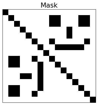
The mask is a boolean array of the same shape as the Hamiltonian, where True values indicate the terms to keep in the Hamiltonian, and False values indicate the terms to cancel.

We apply the mask to the Hamiltonian by providing it as the fully_diagonalize argument to block_diagonalize.

H_tilde, *_ = pymablock.block_diagonalize([H_0, H_1], fully_diagonalize=mask)

The argument fully_diagonalize is a dictionary where the keys label the blocks of the Hamiltonian, and the values are the masks that select the terms to keep in that block. We only used one block in this example.

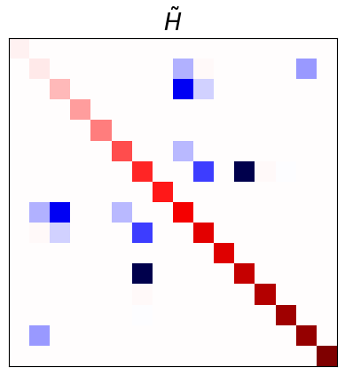
Finally, we plot the transformed Hamiltonian \(\tilde{H}\)

from matplotlib.colors import TwoSlopeNorm

Heff = H_tilde[0, 0, 0] + H_tilde[0, 0, 1] + H_tilde[0, 0, 2]

plt.imshow(Heff, cmap='seismic', norm=TwoSlopeNorm(vcenter=0))
plt.title(r'$\tilde{H}$')
plt.xticks([])
plt.yticks([]);