Comparison to generalized Schrieffer-Wolff transformation

Note

This is an advanced topic both code-wise and conceptually. You do not need to follow this even for advanced uses of Pymablock.

Pymablock computes Hamiltonian’s perturbative series using the least action principle by minimizing \(\|\mathcal{U} - 1\|\). In the two-block case, this is equivalent to the Schrieffer-Wolff transformation. However, in more general cases such as multi-block diagonalization or eliminating arbitrary off-diagonal elements, the Schrieffer-Wolff transformation does not satisfy the least action principle.

In introducing the Pymablock algorithm, we show that it is more efficient and naturally extends to multiple perturbations. A question remains: do these two algorithms have comparable stability and convergence?

To answer this we:

• Implement a prototype selective diagonalization using the Schrieffer-Wolff transformation.

• Compare its convergence properties with those of Pymablock.

Selective diagonalization via Schrieffer-Wolff

The Schrieffer-Wolff transformation uses a unitary of the form \(\exp(\mathcal{S})\), with each order of \(\mathcal{S}\) strictly off-diagonal. Just like in Pymablock algorithm, we eliminate the specified off-diagonal part of \(\tilde{\mathcal{H}} = \exp(\mathcal{S}) \mathcal{H} \exp(-\mathcal{S})\) at each perturbation order by solving for \(\mathcal{S}\) with a Sylvester equation.

From the Baker-Campbell-Hausdorff formula, we have:

\[\exp(\mathcal{S}) \mathcal{H} \exp(-\mathcal{S}) = \mathcal{H} + [\mathcal{S}, \mathcal{H}] + \tfrac{1}{2!} [\mathcal{S}, [\mathcal{S}, \mathcal{H}]] + \ldots.\]

Because \(S_0=0\), the \(n\)-th order of \(\tilde{H}_n\) only contains \(S_n\) through \([S_n, H_0]\). We obtain \(S_n\) from the \(n\)-th order of the remaining terms and solve using the Sylvester equation.

Show code cell source Hide code cell source

from math import factorial

import numpy as np
from matplotlib import pyplot as plt

import pymablock
from pymablock.series import BlockSeries, zero
from pymablock.block_diagonalization import solve_sylvester_diagonal, is_diagonal

np.set_printoptions(precision=2, suppress=True)

def zero_sum(*terms):
    """
    Returns the sum of all non-zero terms, or a singleton zero if no terms exist.
    """
    return sum((term for term in terms if term is not zero), start=zero)

Below is a helper function to compute terms of the Baker–Campbell–Hausdorff series efficiently. This function builds nested commutators of two series, A and B, and avoids direct expansion of nested terms:

def baker_camphell_hausdorff(A: BlockSeries, B: BlockSeries, skip_last=False) -> BlockSeries:
    """
    Compute the series expansion of exp(A) @ B @ exp(-A) using the BCH formula.
    If skip_last is True, the lowest-order terms in the nested commutators are skipped.
    """
    if not (A.n_infinite == B.n_infinite == 1 and A.shape == B.shape == ()):
        raise ValueError("Only 1x1 infinite blocks are supported.")

    # Nested commutators store the m-th order of the n-nested commutator of A and B.
    nested_commutators = BlockSeries(shape=(), n_infinite=2)

    # Define a function to compute entries of the nested_commutators series on demand.
    def nested_commutators_eval(*index):
        n, m = index
        if n > m:
            return zero
        if n == 0:
            return B[m]

        product = zero_sum(
            *(
                A[k] @ nc
                for k in range(1, m + 1)
                if (nc := nested_commutators[n - 1, m - k]) is not zero
                and A[k] is not zero
            )
        )
        # Assume A is anti-Hermitian and B is Hermitian.
        return product + product.T.conj() if product is not zero else zero

    nested_commutators.eval = nested_commutators_eval

    # Build the final BCH series summation.
    def bch_eval(m):
        return zero_sum(
            *(nested_commutators[n, m] * (1 / factorial(n)) for n in range(2 * skip_last, m + 1))
        )

    return BlockSeries(eval=bch_eval, shape=(), n_infinite=1)

The implementation of baker_camphell_hausdorff uses the ability to define BlockSeries recursively by providing an eval function. Specifically, evaluating a block of nested_commutators with index (n, m) uses lower order terms of the same series in its computation.

The following function implements the generalized Schrieffer-Wolff approach, which zeroes out the specified elements of the Hamiltonian (by a binary mask array). Here, it focuses on a single first-order perturbation for simplicity:

def schrieffer_wolff(H_0, H_1, mask):
    """
    Carry out Schrieffer-Wolff diagonalization for a single first-order perturbation.

    H_0 must be diagonal. The 'mask' array indicates which off-diagonal elements to
    eliminate.
    """
    if not is_diagonal(H_0):
        raise ValueError("H_0 must be diagonal")
    solve_sylvester = solve_sylvester_diagonal((np.diag(H_0),))

    # Build series objects
    H = BlockSeries(data={(0,): H_0, (1,): H_1}, n_infinite=1, shape=())
    H_0_series = BlockSeries(data={(0,): H_0}, n_infinite=1, shape=())
    H_p = BlockSeries(data={(0,): zero, (1,): H_1}, n_infinite=1, shape=())
    S = BlockSeries(data={(0,): zero}, n_infinite=1, shape=())

    exp_S_Hp_exp_mS = baker_camphell_hausdorff(S, H_p)
    exp_S_H0_exp_mS = baker_camphell_hausdorff(S, H_0_series, skip_last=True)

    # Define the solver for S at order m.
    def S_eval(m):
        return solve_sylvester(
            zero_sum(exp_S_Hp_exp_mS[m], exp_S_H0_exp_mS[m]) * mask, [0, 0, m]
        )

    S.eval = S_eval
    return baker_camphell_hausdorff(S, H), S

Comparison of the algorithms

First, we confirm correctness in the 2×2 block-diagonalization case by verifying that both approaches give matching results for a random Hamiltonian:

np.random.seed(0)
N = 10
H_0 = np.diag(np.arange(N))
H_1 = np.random.rand(N, N) + 1j * np.random.rand(N, N)
H_1 += H_1.conj().T

# Create a mask for 2x2 block-diagonalization
mask = np.zeros((N, N), dtype=bool)
mask[: N // 2, N // 2 :] = True
mask[N // 2 :, : N // 2] = True

H_tilde, *_ = pymablock.block_diagonalize([H_0, H_1], fully_diagonalize={0: mask})
H_tilde_sw, S = schrieffer_wolff(H_0, H_1, mask)

n = 5
np.testing.assert_almost_equal(H_tilde_sw[n], H_tilde[0, 0, n])

We then compare the convergence properties for different masks:

1. Define a diagonal \(H_0\), a random \(H_1\), and a chosen mask.

2. Construct \(H_0 + \alpha H_1\) for varying \(\alpha\), apply both methods up to a certain perturbation order, and compare the eigenvalues with exact ones.

3. Compute and plot the ratio of errors vs. exact energies.

Show code cell source Hide code cell source

import time

def compare_schrieffer_wolff_pymablock(
    H_0, H_1, mask, n_max=100, alpha_max=0.5, title=""
):
    """
    Compare the Schrieffer-Wolff and Pymablock algorithms by looking at the
    difference between approximate and exact eigenvalues as alpha varies.
    """
    # Use Pymablock's block_diagonalize to get the standard approach.
    H_tilde, *_ = pymablock.block_diagonalize([H_0, H_1], fully_diagonalize={0: mask})

    # Use our Schrieffer-Wolff approach.
    H_tilde_sw, S = schrieffer_wolff(H_0, H_1, mask)

    alpha = np.linspace(0, alpha_max, 100).reshape(1, 1, 1, -1)
    powers = np.arange(n_max).reshape(-1, 1, 1, 1)

    # Convert the resulting series objects to arrays for easier operations.
    start_time = time.time()
    H_orders = H_tilde[0, 0, :n_max]
    H_orders[0] = H_0  # Overwrite zeroth order with the exact H_0
    time_H_orders = time.time() - start_time

    start_time = time.time()
    H_orders_sw = H_tilde_sw[:n_max]
    time_H_orders_sw = time.time() - start_time

    # Compute approximate and exact eigenvalues.
    eigvals_la = np.linalg.eigvalsh(
        np.cumsum(np.array(list(H_orders))[..., None] * alpha**powers, axis=0).transpose(
            0, 3, 1, 2
        )
    )
    eigvals_sw = np.linalg.eigvalsh(
        np.cumsum(
            np.array(list(H_orders_sw))[..., None] * alpha**powers, axis=0
        ).transpose(0, 3, 1, 2)
    )
    eigvals_exact = np.linalg.eigvalsh(
        (H_0[..., None] + H_1[..., None] * alpha[0, 0, 0]).transpose(2, 0, 1)
    )[None, ...]

    # Create plots for error norms
    fig = plt.figure(layout="constrained")
    ax1, ax2 = fig.subplots(2, 1, sharex=True)

    for order in range(n_max):
        la_err = np.linalg.norm(eigvals_la[order] - eigvals_exact, axis=(0, -1))
        sw_err = np.linalg.norm(eigvals_sw[order] - eigvals_exact, axis=(0, -1))
        ratio = np.divide(sw_err, la_err, out=np.zeros_like(sw_err), where=la_err != 0)

        ax1.plot(alpha.flatten()[1:], la_err[1:], c=plt.cm.inferno(order / n_max))
        ax2.plot(alpha.flatten()[1:], ratio[1:], c=plt.cm.inferno(order / n_max))

    ax1.set_ylabel("Error Pymablock")
    ax1.set_title(title)
    ax2.set_ylabel(
        " Error SW / Error Pymablock"
    )
    ax2.set_title(f"Time Pymablock {time_H_orders:.2f}s, Time SW: {time_H_orders_sw:.2f}s")
    ax2.set_xlabel(r"$\alpha$")
    for ax in (ax1, ax2):
        ax.semilogy()

    # Display the mask in an inset
    inset_ax = fig.add_axes([0.15, 0.75, 0.2, 0.2])
    inset_ax.imshow(mask, cmap="gray", interpolation="none")
    inset_ax.set_xticks([])
    inset_ax.set_yticks([])

    # Add a colorbar to indicate the perturbation order
    cbar = fig.colorbar(
        plt.cm.ScalarMappable(cmap="inferno", norm=plt.Normalize(vmin=0, vmax=n_max)),
        ax=[ax1, ax2],
        orientation="vertical",
    )
    cbar.set_label("Order")

Finally, we are ready to compare the convergence properties for different patterns of eliminated matrix elements.

First, we consider a random mask:

Show code cell source Hide code cell source

np.random.seed(2)
N = 9
H_0 = np.diag(10 * np.random.randn(N))
H_1 = np.random.rand(N, N) + 1j * np.random.rand(N, N)
H_1 += H_1.conj().T

mask = np.random.rand(N, N) < 0.3
mask = mask | mask.T
mask = mask & ~np.eye(N, dtype=bool)

compare_schrieffer_wolff_pymablock(
    H_0, H_1, mask, n_max=30, alpha_max=2, title="Random Mask"
)

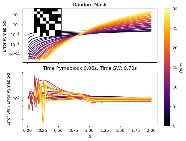
Let us unpack what we see here:

• We are eliminating the matrix elements shown with the white color in the inset.

• In the top panel at low \(\alpha\), the error of the Pymablock algorithm drops with the order of perturbation (line color): we are below the convergence radius.

• At high \(\alpha\), the error starts diverging faster and faster with order, and the transition between the two regimes is the convergence radius of the series.

• Regardless of whether \(\alpha\) is high or low, the bottom panel shows that the ratio between two errors stays roughly constant as a function of the perturbation order.

• While the errors behave similarly, the time taken by the algorithms is vastly different: Pymablock is faster by more than an order of magnitude.

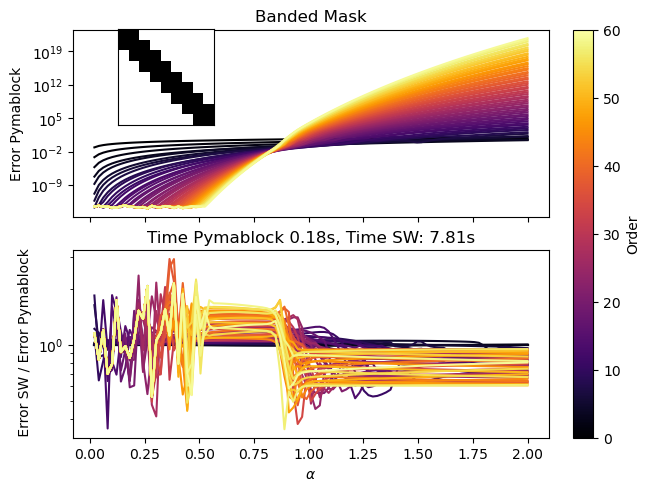
For completeness, let us also consider other masks. Here we take a banded mask where we eliminate all off-diagonal elements outside of a width-3 band:

Show code cell source Hide code cell source

banded_mask = np.ones((N, N), dtype=bool)
for k in range(-1, 2):
    banded_mask ^= np.eye(N, k=k, dtype=bool)

compare_schrieffer_wolff_pymablock(
    H_0, H_1, banded_mask, n_max=60, alpha_max=2, title="Banded Mask"
)

Finally, we consider 3×3 block-diagonalization:

Show code cell source Hide code cell source

three_block_mask = np.ones((N, N), dtype=bool)
slices = [slice(None, N // 3), slice(N // 3, 2 * N // 3), slice(2 * N // 3, None)]
for s in slices:
    three_block_mask[s, s] = False

compare_schrieffer_wolff_pymablock(
    H_0,
    H_1,
    three_block_mask,
    n_max=100,
    alpha_max=2,
    title="3x3 Block-Diagonalization Mask",
)

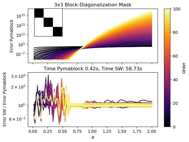
We observe that in all cases both approaches exhibit similar radii of convergence and overall error behavior—a fact for which we don’t have an explanation so far. Still, just like we expected, the Pymablock algorithm is much faster.