The algorithm

Problem formulation

Pymablock finds a series of the unitary transformation \(\mathcal{U}\) (we use calligraphic letters to denote series) that block-diagonalizes the Hamiltonian

(1)\[\begin{split}\mathcal{H} = H_0 + \mathcal{H}',\quad H_0 = \begin{pmatrix} H_0^{AA} & 0\\ 0 & H_0^{BB} \end{pmatrix},\end{split}\]

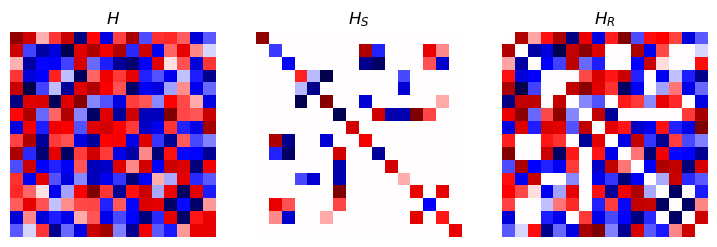
with \(\mathcal{H}' = \mathcal{H}'_{D} + \mathcal{H}'_{O}\) containing an arbitrary number and orders of perturbations with block-diagonal and block-offdiagonal components, respectively. The series here may be multivariate, and they represent sums of the form

\[ \mathcal{A} = \sum_{n_1=0}^\infty \sum_{n_2=0}^\infty \cdots \sum_{n_k=0}^\infty \lambda_1^{n_1} \lambda_2^{n_2} \cdots \lambda_k^{n_k} A_{n_1, n_2, \ldots, n_k}, \]

where \(\lambda_i\) are the perturbation parameters and \(A_{n_1, n_2, \ldots, n_k}\) are linear operators.

The problem statement, therefore, is finding \(\mathcal{U}\) and \(\tilde{\mathcal{H}}\) such that:

(2)\[\tilde{\mathcal{H}} = \mathcal{U}^\dagger \mathcal{H} \mathcal{U},\quad \tilde{\mathcal{H}}^{AB} = 0,\quad \mathcal{U}^\dagger \mathcal{U} = 1,\]

where series multiply according to the Cauchy product:

\[ \mathcal{C} = \mathcal{A}\mathcal{B} \Leftrightarrow C_\mathbf{n} = \sum_{\mathbf{m} + \mathbf{p} = \mathbf{n}} A_\mathbf{m} B_\mathbf{p}. \]

Computational complexity of the Cauchy product

The Cauchy product is the most expensive operation in perturbation theory, because it involves a large number of multiplications between potentially large matrices, so let us discuss its complexity. Evaluating \(\mathbf{n}\)-th order of \(\mathcal{C}\) requires \(\sim\prod_i n_i = N\) multiplications of the series elements. A direct computation of all the possible index combinations in a product between three series \(\mathcal{A}\mathcal{B}\mathcal{C}\) would have a higher cost \(\sim N^2\), however if we use associativity of the product and compute this as \((\mathcal{A}\mathcal{B})\mathcal{C}\), then the scaling of the cost stays \(\sim N\).

How to solve the problem?

There are many ways to solve this problem that give identical expressions for \(\mathcal{U}\) and \(\tilde{\mathcal{H}}\). We are searching for a procedure that satisfies three additional constraints:

• It has the same complexity scaling as a Cauchy product.

• It does not require multiplications by \(H_0\). This is because in perturbation theory, \(n\)-th order corrections to \(\tilde{\mathcal{H}}\) carry \(n\) energy denominators \(1/(E_i - E_j)\) (see here). Therefore, any additional multiplications by \(H_0\) must cancel with additional energy denominators. Multiplying by \(H_0\) is therefore unnecessary work, and it gives longer intermediate expressions.

• It requires only one Cauchy product by \(\mathcal{H}_D\), the block-diagonal part of \(\mathcal{H}\). By considering \(\mathcal{H}_{O}=0\), we observe that \(\mathcal{H}_D\) must at least enter \(\tilde{\mathcal{H}}\) as an added term, without any products. Moreover, because \(\mathcal{U}\) depends on the entire Hamiltonian, there must be at least one Cauchy product by \(\mathcal{H}'_D\). This lower bound turns out to be possible to achieve.

The goal of our algorithm is thus to be efficient and to produce compact results that do not require further simplifications.

Our solution

To find \(\mathcal{U}\), let us separate it into an identity and \(\mathcal{U}' = \mathcal{W} + \mathcal{V}\):

(3)\[\mathcal{U} = 1 + \mathcal{U}' = 1 + \mathcal{W} + \mathcal{V},\quad \mathcal{W}^\dagger = \mathcal{W},\quad \mathcal{V}^\dagger = -\mathcal{V}.\]

First, we use the unitarity condition \(\mathcal{U}^\dagger \mathcal{U} = 1\) by substituting \(\mathcal{U}'\) into it and obtain

(4)\[\begin{split}\toggle{ \mathcal{W} = \texttip{\color{red}{\ldots}}{click to expand} = -\frac{1}{2} \mathcal{U}'^\dagger \mathcal{U}'. }{ \begin{align} \mathcal{W} &= \frac{1}{2}(\mathcal{U}'^\dagger + \mathcal{U}') \\ &= \frac{1}{2} \Big[(1 + \mathcal{U}'^\dagger)(1+\mathcal{U}') - 1 - \mathcal{U}'^\dagger \mathcal{U}' \Big] \\ &= -\frac{1}{2} \mathcal{U}'^\dagger \mathcal{U}'. \end{align} } \endtoggle\end{split}\]

Because \(\mathcal{U}'\) has no \(0\)-th order term, \((\mathcal{U}'^\dagger \mathcal{U}')_\mathbf{n}\) does not depend on the \(\mathbf{n}\)-th order of \(\mathcal{U}'\) nor \(\mathcal{W}\). More generally, a Cauchy product \(\mathcal{A}\mathcal{B}\) where \(\mathcal{A}\) and \(\mathcal{B}\) have no \(0\)-th order terms depends on \(\mathcal{A}_1, \ldots, \mathcal{A}_{n-1}\) and \(\mathcal{B}_1, \ldots, \mathcal{B}_{n-1}\). This allows us to use Cauchy products to define recurrence relations, which we apply throughout the algorithm. Therefore, we compute \(\mathcal{W}\) as a Cauchy product of \(\mathcal{U}'\) with itself. This recurrence relation is the first secret ingredient of Pymablock✨

Choosing the right definition for \(\mathcal{W}\)

Using the definition of \(\mathcal{W}\) as the Hermitian part of \(\mathcal{U}'\), and the unitarity condition:

\[ \begin{align} 2\mathcal{W} = \mathcal{U}' + \mathcal{U}'^\dagger = -\mathcal{U}'^\dagger \mathcal{U}' = -\mathcal{W}^2 + \mathcal{V}^2. \end{align} \]

we see that we could alternatively define \(\mathcal{W}\) as a Taylor series in \(\mathcal{V}\):

\[ \mathcal{W} = \sqrt{1 + \mathcal{V}^2} - 1 \equiv f(\mathcal{V}) \equiv \sum_n a_n \mathcal{V}^{2n}, \]

however the scaling of such a Cauchy product becomes slower if we need to compute a Taylor expansion of a series:

\[ f(\mathcal{A}) = \sum_{n=0}^\infty a_n \mathcal{A}^n. \]

However, evaluating a Taylor expansion of a given series has a higher scaling of complexity. A direct computation of all possible products of terms would require \(\sim \exp N\) multiplications. We improve on this by defining a new series as \(\mathcal{A}^{n+1} = \mathcal{A}\mathcal{A}^{n}\) and reusing the previously computed results, which brings these costs down to \(\sim N^2\). Using the Taylor expansion approach is therefore both more complicated and more computationally expensive than the recurrent definition in (4).

To compute \(\mathcal{U}'\) we also need to find \(\mathcal{V}\), which is defined by the requirement \(\tilde{\mathcal{H}}^{AB} = 0\). Additionally, we constrain \(\mathcal{V}\) to be block off-diagonal: \(\mathcal{V}^{AA} = \mathcal{V}^{BB} = 0\), so that the resulting unitary transformation is equivalent to the Schrieffer-Wolff transformation. In turn, this means that \(\mathcal{W}\) is block-diagonal and that the norm of \(\mathcal{U}'\) is minimal.

Equivalence to Schrieffer-Wolff transformation

Both the Pymablock algorithm and the more commonly used Schrieffer-Wolfftr ansformation find a unitary transformation \(\mathcal{U}\) such that \(\tilde{\mathcal{H}}^{AB}=0\). They are therefore equivalent up to a gauge choice in each subspace, \(A\) and \(B\). We establish the equivalence between the two by demonstrating that this gauge choice is the same for both algorithms.

The Schrieffer-Wolff transformation uses \(\mathcal{U} = \exp \mathcal{S}\), where \(\mathcal{S} = -\mathcal{S}^\dagger\) and \(\mathcal{S}^{AA} = \mathcal{S}^{BB} = 0\).

The series \(\exp\mathcal{S}\) contains all possible products of \(S_n\) of all lengths with fractional prefactors. For every term \(S_{k_1}S_{k_2}\cdots S_{k_n}\), there is a corresponding term \(S_{k_n}S_{k_{n-1}}\cdots S_{k_1}\) with the same prefactor. If the number of \(S_{k_n}\) is even, then both terms are block-diagonal since each \(S_n\) is block off-diagonal. Because \(S_n\) are anti-Hermitian, the two terms are Hermitian conjugates of each other, and therefore their sum is Hermitian. On the other hand, if the number of \(S_{k_n}\) is odd, then the two terms are block off-diagonal and their sum is anti-Hermitian by the same reasoning.

Therefore, just like in our algorithm, the diagonal blocks of \(\exp S\) are Hermitian, while off-diagonal blocks are anti-Hermitian. Schrieffer-Wolff transformation produces a unique answer and satisfies the same diagonalization requirements as our algorithm, which means that the two are equivalent.

To find \(\mathcal{V}\), we need to first look at the transformed Hamiltonian:

\[ \tilde{\mathcal{H}} = \mathcal{U}^\dagger \mathcal{H} \mathcal{U} = \mathcal{H}_D + \mathcal{U}'^\dagger \mathcal{H}_D + \mathcal{H}_D \mathcal{U}' + \mathcal{U}'^\dagger \mathcal{H}_D \mathcal{U}' + \mathcal{U}^\dagger\mathcal{H}'_{O}\mathcal{U}, \]

where we used \(\mathcal{U}=1+\mathcal{U}'\) and \(\mathcal{H} = \mathcal{H}_D + \mathcal{H}'_{O}\), since \(H_0\) is block-diagonal by definition.

Because we want to avoid unnecessary products by \(\mathcal{H}_D\), we need to get rid of the terms that contain it by replacing them with an alternative expression. Our strategy is to define an auxiliary operator \(\mathcal{X}\) that we can compute without ever multiplying by \(\mathcal{H}_D\). Like \(\mathcal{U}'\), \(\mathcal{X}\) needs to be defined via a recurrence relation, which we will find later. Because the expression above has \(\mathcal{H}_D\) multiplied by \(\mathcal{U}'\) by the left and by the right, we get rid of these terms by making sure that \(\mathcal{H}_D\) multiplies terms from one side only. To achieve this, we choose \(\mathcal{X}=\mathcal{Y}+\mathcal{Z}\) to be the commutator between \(\mathcal{U}'\) and \(\mathcal{H}_D\):

(5)\[\mathcal{X} \equiv [\mathcal{U}', \mathcal{H}_D] = \mathcal{Y} + \mathcal{Z}, \quad \mathcal{Y} \equiv [\mathcal{V}, \mathcal{H}_D] = \mathcal{Y}^\dagger,\quad \mathcal{Z} \equiv [\mathcal{W}, \mathcal{H}_D] = -\mathcal{Z}^\dagger,\]

where \(\mathcal{Y}\) is therefore block off-diagonal and \(\mathcal{Z}\), block diagonal. We use \(\mathcal{H}_D \mathcal{U}' = \mathcal{U}' \mathcal{H}_D -\mathcal{X}\) to move \(\mathcal{H}_D\) through to the right and find

(6)\[\begin{split}\toggle{ \tilde{\mathcal{H}} = \texttip{\color{red}{\ldots}}{click to expand} = \mathcal{H}_D - \mathcal{X} - \mathcal{U}'^\dagger \mathcal{X} + \mathcal{U}^\dagger\mathcal{H}'_{O}\mathcal{U}, }{ \begin{align*} \tilde{\mathcal{H}} &= \mathcal{H}_D + \mathcal{U}'^\dagger \mathcal{H}_D + (\mathcal{H}_D \mathcal{U}') + \mathcal{U}'^\dagger \mathcal{H}_D \mathcal{U}' + \mathcal{U}^\dagger\mathcal{H}'_{O}\mathcal{U} \\ &= \mathcal{H}_D + \mathcal{U}'^\dagger \mathcal{H}_D + \mathcal{U}'\mathcal{H}_D - \mathcal{X} + \mathcal{U}'^\dagger (\mathcal{U}' \mathcal{H}_D - \mathcal{X}) + \mathcal{U}^\dagger\mathcal{H}_{O}\mathcal{U}\\ &= \mathcal{H}_D + (\mathcal{U}'^\dagger + \mathcal{U}' + \mathcal{U}'^\dagger \mathcal{U}')\mathcal{H}_D - \mathcal{X} - \mathcal{U}'^\dagger \mathcal{X} + \mathcal{U}^\dagger\mathcal{H}'_{O}\mathcal{U}\\ &= \mathcal{H}_D - \mathcal{X} - \mathcal{U}'^\dagger \mathcal{X} + \mathcal{U}^\dagger\mathcal{H}'_{O}\mathcal{U}, \end{align*} } \endtoggle\end{split}\]

where the terms multiplied by \(\mathcal{H}_D\) cancel by unitarity.

The transformed Hamiltonian does not contain products by \(\mathcal{H}_D\) anymore, but it does depend on \(\mathcal{X}\), an auxiliary operator whose recurrent definition we do not know yet. To find it, we first focus on its anti-Hermitian part, \(\mathcal{Z}\). Since recurrence relations are expressions whose right hand side contains Cauchy products between series, we need to find a way to make a product appear. This is where the unitarity condition \(\mathcal{U}'^\dagger + \mathcal{U}' = -\mathcal{U}'^\dagger \mathcal{U}'\) comes in handy and gives:

(7)\[\begin{split}\toggle{ \mathcal{Z} = \texttip{\color{red}{\ldots}}{click to expand} = \frac{1}{2}(-\mathcal{U}'^\dagger\mathcal{X} + \mathcal{X}^\dagger\mathcal{U}'). }{ \begin{align} \mathcal{Z} &= \frac{1}{2} (\mathcal{X} - \mathcal{X}^{\dagger}) \\ &= \frac{1}{2}\Big[ (\mathcal{U}' + \mathcal{U}'^{\dagger}) \mathcal{H}_D - \mathcal{H}_D (\mathcal{U}' + \mathcal{U}'^{\dagger}) \Big] \\ &= \frac{1}{2} \Big[ - \mathcal{U}'^{\dagger} (\mathcal{U}'\mathcal{H}_D - \mathcal{H}_D \mathcal{U}') + (\mathcal{U}'\mathcal{H}_D - \mathcal{H}_D \mathcal{U}')^{\dagger} \mathcal{U}' \Big] \\ &= \frac{1}{2} (-\mathcal{U}'^{\dagger} \mathcal{X} + \mathcal{X}^{\dagger} \mathcal{U}'). \end{align} } \endtoggle\end{split}\]

Similar to computing \(W_\mathbf{n}\), computing \(Z_\mathbf{n}\) requires lower orders of \(\mathcal{X}\) and \(\mathcal{U}'\), all blocks included. This is our second secret ingredient✨

Then, we compute the Hermitian part of \(\mathcal{X}\) by requiring that \(\tilde{\mathcal{H}}^{AB} = 0\) and find

(8)\[\mathcal{X}^{AB} = (\mathcal{U}^\dagger \mathcal{H}'_{O} \mathcal{U} - \mathcal{U}'^\dagger \mathcal{X})^{AB}.\]

Once again, despite \(\mathcal{X}\) enters the right hand side, because all the terms lack 0-th order, this defines a recursive relation for \(\mathcal{X}^{AB}\), and therefore \(\mathcal{Y}\). This is our last secret ingredient✨

The final part is straightforward: the definition of \(\mathcal{Y}\) in (5) fixes \(\mathcal{V}\) as a solution of:

(9)\[\mathcal{V}^{AB}H_0^{BB} - H_0^{AA} \mathcal{V}^{AB} = \mathcal{Y}^{AB} - [\mathcal{V}, \mathcal{H}'_D]^{AB},\]

a Sylvester’s equation, which we only need to solve once for every new order. This is the only step in the algorithm that requires a direct multiplication by \(\mathcal{H}'_D\). In the eigenbasis of \(H_0\), the solution of Sylvester’s equation is \(V^{AB}_{\mathbf{n}, ij} = (\mathcal{Y} - [\mathcal{V}, \mathcal{H}'_D])^{AB}_{\mathbf{n}, ij}/(E_i - E_j)\), where \(E_i\) are the eigenvalues of \(H_0\). However, even if the eigenbasis of \(H_0\) is not available, there are efficient algorithms to solve Sylvester’s equation, see below.

Actual algorithm

We now have the complete algorithm:

1. Define series \(\mathcal{U}'\) and \(\mathcal{X}\) and make use of their block structure and Hermiticity.

2. To define the diagonal blocks of \(\mathcal{U}'\), use \(\mathcal{W} = -\mathcal{U}'^\dagger\mathcal{U}'/2\).

3. To find the off-diagonal blocks of \(\mathcal{U}'\), solve Sylvester’s equation \(\mathcal{V}^{AB}H_0^{BB} - H_0^{AA}\mathcal{V}^{AB} = \mathcal{Y}^{AB} - [\mathcal{V}, \mathcal{H}'_D]\). This requires \(\mathcal{X}\).

4. To find the diagonal blocks of \(\mathcal{X}\), define \(\mathcal{Z} = (-\mathcal{U}'^\dagger\mathcal{X} + \mathcal{X}^\dagger\mathcal{U}')/2\).

5. For the off-diagonal blocks of \(\mathcal{X}\), use \(\mathcal{Y}^{AB} = (-\mathcal{U}'^\dagger\mathcal{X} + \mathcal{U}^\dagger\mathcal{H}'_{O}\mathcal{U})^{AB}\).

6. Compute the effective Hamiltonian as \(\tilde{\mathcal{H}}_{D} = \mathcal{H}_D - \mathcal{X} - \mathcal{U}'^\dagger \mathcal{X} + \mathcal{U}^\dagger\mathcal{H}'_{O}\mathcal{U}\).

Extra optimization: common subexpression elimination

We further optimize the algorithm by reusing products that are needed in several places.

Firstly, we rewrite the expressions for \(\mathcal{Z}\) and \(\tilde{\mathcal{H}}\) by utilizing the Hermitian conjugate of \(\mathcal{U}'^\dagger \mathcal{X}\) without recomputing it:

\[\begin{split} \begin{gather*} \mathcal{Z} = \frac{1}{2}[(-\mathcal{U}'^\dagger \mathcal{X})- \textrm{h.c.}],\\ \tilde{\mathcal{H}} = \mathcal{H}_D + \mathcal{U}^\dagger \mathcal{H}'_{O} \mathcal{U} - (\mathcal{U}'^\dagger \mathcal{X} + \textrm{h.c.})/2, \end{gather*} \end{split}\]

where \(\textrm{h.c.}\) is the Hermitian conjugate, and \(\mathcal{X}\) drops out from the diagonal blocks of \(\tilde{\mathcal{H}}\) because diagonal of \(\mathcal{X}\) is anti-Hermitian.

To compute \(\mathcal{U}^\dagger \mathcal{H}'_{O} \mathcal{U}\) faster, we express it using \(\mathcal{A} \equiv \mathcal{H}'_{O}\mathcal{U}'\):

\[ \mathcal{U}^\dagger \mathcal{H}'_{O} \mathcal{U} = \mathcal{H}'_{O} + \mathcal{A} + \mathcal{A}^\dagger + \mathcal{U}'^\dagger \mathcal{A}. \]

To further optimize the computations, we observe that some products appear both in \(\mathcal{U}'^\dagger \mathcal{X}\) and \(\mathcal{U}^\dagger \mathcal{H}'_{O} \mathcal{U}\). We reuse these products by introducing \(\mathcal{B} = \mathcal{X} - \mathcal{H}'_{O} - \mathcal{A}\).

Using this definition, we first express the off-diagonal blocks of \(\mathcal{B}\) as follows:

\[\begin{split} \toggle{ \mathcal{B}^{AB, BA} = \texttip{\color{red}{\ldots}}{click to expand} = -(\mathcal{U'}^\dagger \mathcal{B})^{AB, BA}, }{ \begin{align*} \mathcal{B}^{AB, BA} &= \left[\mathcal{X} - \mathcal{H}'_{O} - \mathcal{A} \right]^{AB, BA}\\ &= \left[\mathcal{A}^\dagger + \mathcal{U}'^\dagger\mathcal{A} - \mathcal{U}'^\dagger \mathcal{X} \right]^{AB, BA}\\ &= \left[\mathcal{U}'^\dagger\mathcal{H}'_{O} + \mathcal{U}'^\dagger\mathcal{A} - \mathcal{U}'^\dagger \mathcal{X} \right]^{AB, BA}\\ &= -(\mathcal{U'}^\dagger \mathcal{B})^{AB, BA}, \end{align*} } \endtoggle \end{split}\]

where we also used Eq. (8) and the definition of \(\mathcal{A}\).

Its diagonal blocks, on the other hand, are given by

\[\begin{split} \toggle{ \mathcal{B}^{AA, BB} = \texttip{\color{red}{\ldots}}{click to expand} = \left[\frac{1}{2}[(-\mathcal{U}'^\dagger \mathcal{B})- \textrm{h.c.}] - \frac{1}{2}[\mathcal{A}^\dagger + \mathcal{A} ]\right]^{AA, BB}, }{ \begin{align*} \mathcal{B}^{AA, BB} &= \left[\mathcal{X} - \mathcal{H}'_{O} - \mathcal{A}\right]^{AA, BB} \\ &= \left[\frac{1}{2}[(-\mathcal{U}'^\dagger \mathcal{X})- \textrm{h.c.}] - \mathcal{A}\right]^{AA, BB} \\ &= \left[\frac{1}{2}[(-\mathcal{U}'^\dagger [\mathcal{X} - \mathcal{H}'_{O} - \mathcal{A}])- \textrm{h.c.}] - \frac{1}{2}[\mathcal{A}^\dagger + \mathcal{A} ] + {\frac{1}{2}[( - \mathcal{U}'^\dagger\mathcal{A} ) - \textrm{h.c.}]}\right]^{AA, BB}, \\ &= \left[\frac{1}{2}[(-\mathcal{U}'^\dagger \mathcal{B})- \textrm{h.c.}] - \frac{1}{2}[\mathcal{A}^\dagger + \mathcal{A} ]\right]^{AA, BB}, \end{align*} } \endtoggle \end{split}\]

where we used Eq. (7) and that the \(\mathcal{U}'^\dagger \mathcal{A}\) is Hermitian.

Finally, we compute the diagonal part of \(\tilde{\mathcal{H}}\) as

\[ \tilde{\mathcal{H}}_D = \mathcal{H}_D + (\mathcal{A} + \mathcal{A}^\dagger)/2 -(\mathcal{U}^\dagger \mathcal{B} + \textrm{h.c.})/2. \]

How to use Pymablock on large numerical Hamiltonians?

Solving Sylvester’s equation and computing the matrix products are the most expensive steps of the algorithms for large Hamiltonians. Pymablock can efficiently construct an effective Hamiltonian of a small subspace even when the full Hamiltonian is a sparse matrix that is too costly to diagonalize. It does so by avoiding explicit computation of operators in \(B\) subspace, and by utilizing the sparsity of the Hamiltonian to compute the Green’s function. To do so, Pymablock uses either the MUMPS sparse solver via the python-mumps wrapper or the KPM method.

This approach was originally introduced in this work.

Implementation details

We use the matrix \(\Psi_A\) of the eigenvectors of the \(A\) subspace to rewrite the Hamiltonian as

\[\begin{split}\mathcal{H} \to \begin{pmatrix} \Psi_A^\dagger \mathcal{H} \Psi_A & \Psi_A^\dagger \mathcal{H} P_B \\ P_B \mathcal{H} \Psi_A & P_B \mathcal{H} P_B \end{pmatrix},\end{split}\]

where \(P_B = 1 - \Psi_A \Psi_A^\dagger\) is the projector onto the \(B\) subspace. This Hamiltonian is larger in size than the original one because the \(B\) block has additional null vectors corresponding to the \(A\) subspace. This, however, allows to preserve the sparsity structure of the Hamiltonian by applying \(P_B\) and \(\mathcal{H}\) separately. Additionally, applying \(P_B\) is efficient because \(\Psi_A\) is a low rank matrix. We then perform perturbation theory of the rewritten \(\mathcal{H}\).

To solve the Sylvester’s equation for the modified Hamiltonian, we write it for every row of \(V_{\mathbf{n}}^{AB}\) separately:

\[V_{\mathbf{n}, ij}^{AB} (E_i - H_0) = Y_{\mathbf{n}, j}\]

This equation is well-defined despite \(E_i - H_0\) is not invertible because \(Y_{\mathbf{n}}\) has no components in the \(A\) subspace.