Induced gap in a double quantum dot#
This tutorial demonstrates how to efficiently build effective models from big numerical Hamiltonians. It also shows how Pymablock integrates with Kwant. As an example, we consider a tight binding model of a quantum dot and a superconductor with a tunnel barrier in between.
Let’s start by importing the necessary packages
import tinyarray as ta
import matplotlib.backends
import scipy.linalg
from scipy.sparse.linalg import eigsh
import numpy as np
import kwant
import matplotlib.pyplot as plt
color_cycle = ["#5790fc", "#f89c20", "#e42536"]

from pymablock import block_diagonalize
Building the Hamiltonian with Kwant#
Following Kwant’s tutorials we start by defining the lattice
sigma_z = ta.array([[1, 0], [0, -1]], float)
sigma_x = ta.array([[0, 1], [1, 0]], float)

syst = kwant.Builder()
lat = kwant.lattice.square(norbs=2)
L, W = 200, 40
Next, we define the onsite potential for the quantum dot and superconductor
def normal_onsite(site, mu_n, t):
    return (-mu_n + 4 * t) * sigma_z

def sc_onsite(site, mu_sc, Delta, t):
    return (-mu_sc + 4 * t) * sigma_z + Delta * sigma_x

syst[lat.shape((lambda pos: abs(pos[1]) < W and abs(pos[0]) < L), (0, 0))] = normal_onsite
syst[lat.shape((lambda pos: abs(pos[1]) < W and abs(pos[0]) < L / 3), (0, 0))] = sc_onsite
and the hoppings
syst[lat.neighbors()] = lambda site1, site2, t: -t * sigma_z

def barrier(site1, site2):
    return (abs(site1.pos[0]) - L / 3) * (abs(site2.pos[0]) - L / 3) < 0

syst[(hop for hop in syst.hoppings() if barrier(*hop))] = (
    lambda site1, site2, t_barrier: -t_barrier * sigma_z
)
here we make the hoppings between the quantum dots and superconductor equal to t_barrier.
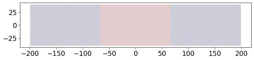
We can now plot the system and finalize it
kwant.plot(
    syst,
    fig_size=(10, 6),
    site_color=(lambda site: abs(site.pos[0]) < L / 3),
    colorbar=False,
    cmap="seismic",
    hop_lw=0,
)

syst = syst.finalized()
f"The system has {len(syst.sites)} sites."
/home/docs/checkouts/readthedocs.org/user_builds/pymablock/checkouts/latest/.pixi/envs/docs/lib/python3.13/site-packages/kwant/_plotter.py:77: RuntimeWarning: plotly is not available, if other engines are unavailable, only iterator-providing functions will work
  warnings.warn("plotly is not available, if other engines are unavailable,"
'The system has 31521 sites.'
In the plot the blue regions are the left and right quantum dots, while the superconductor is the red region in the middle.
We see that the system is large: with this many sites even storing all the eigenvectors would take 60 GB of memory. We must therefore use sparse matrices, and may only compute a few eigenvectors. In this case, perturbation theory allows us to compute the effective Hamiltonian of the low energy degrees of freedom.
To get the unperturbed Hamiltonian, we use the following values for \(\mu_n\), \(\mu_{sc}\), \(\Delta\), \(t\), and \(t_{\text{barrier}}\).
params = dict(
    mu_n=0.05,
    mu_sc=0.3,
    Delta=0.05,
    t=1.,
    t_barrier=0.,
)

h_0 = syst.hamiltonian_submatrix(params=params, sparse=True).real
The barrier strength and the asymmetry of the dot potentials are the two perturbations that we vary.
barrier = syst.hamiltonian_submatrix(
    params={**{p: 0 for p in params.keys()}, "t_barrier": 1}, sparse=True
).real
delta_mu = (
    kwant.operator.Density(syst, (lambda site: sigma_z * site.pos[0] / L)).tocoo().real
)
Define the perturbative series#
In the implicit mode, Pymablock computes the perturbative series without knowing the eigenvectors of one of the Hamiltonian subspaces.
Therefore we compute 4 eigenvectors of the unperturbed Hamiltonian, which correspond to the 4 lowest eigenvalues closest to \(E=0\). These are the lowest energy Andreev states in two quantum dots.
%%time

vals, vecs = eigsh(h_0, k=4, sigma=0)
vecs, _ = scipy.linalg.qr(vecs, mode="economic")  # orthogonalize the vectors
CPU times: user 681 ms, sys: 36 ms, total: 717 ms
Wall time: 717 ms
Note
The orthogonalization is often necessary to do manually because ~scipy.sparse.linalg.eigsh does not return orthogonal eigenvectors if the matrix is complex and eigenvalues are degenerate.
We now define the block diagonalization routine and compute the few lowest orders of the effective Hamiltonian. Here we only provide the set of vectors of the interesting subspace.
%%time

H_tilde, *_ = block_diagonalize([h_0, barrier, delta_mu], subspace_eigenvectors=[vecs])
CPU times: user 536 ms, sys: 43.9 ms, total: 580 ms
Wall time: 580 ms
Block diagonalization is now the most time consuming step because it requires pre-computing several decomposition of the full Hamiltonian. It is, however, manageable and it only produces a constant overhead.
Get results#
For convenience, we collect the lowest three orders in each parameter in an appropriately sized tensor.
%%time

# Combine all the perturbative terms into a single 4D array
fill_value = np.zeros((), dtype=object)
fill_value[()] = np.zeros_like(H_tilde[0, 0, 0, 0])
h_tilde = np.array(np.ma.filled(H_tilde[0, 0, :3, :3], fill_value).tolist())
CPU times: user 398 ms, sys: 20 ms, total: 418 ms
Wall time: 418 ms
We see that we have obtained the effective model in only a few seconds. We can now compute the low energy spectrum after rescaling the perturbative corrections by the magnitude of each perturbation.
def effective_energies(h_tilde, barrier, delta_mu):
    barrier_powers = barrier ** np.arange(3).reshape(-1, 1, 1, 1)
    delta_mu_powers = delta_mu ** np.arange(3).reshape(1, -1, 1, 1)
    return scipy.linalg.eigvalsh(
        np.sum(h_tilde * barrier_powers * delta_mu_powers, axis=(0, 1))
    )
Finally, we plot the spectrum
Show code cell source
%%time

barrier_vals = np.array([0, 0.5, .75])
delta_mu_vals = np.linspace(0, 10e-4, num=101)
results = [
    np.array([effective_energies(h_tilde, bar, dmu) for dmu in delta_mu_vals])
    for bar in barrier_vals
]

plt.figure(figsize=(10, 6), dpi=200)
[
    plt.plot(delta_mu_vals, result, color=color, label=[f"$t_b={barrier}$"] + 3 * [None])
    for result, color, barrier in zip(results, color_cycle, barrier_vals)
]
plt.xlabel(r"$\delta_\mu$")
plt.ylabel(r"$E$")
plt.legend();
CPU times: user 13.6 ms, sys: 58 μs, total: 13.6 ms
Wall time: 13.5 ms

As expected, the crossing at \(E=0\) due to the dot asymmetry is lifted when the dots are coupled to the superconductor. In addition, we observe how the proximity gap of the dots increases with the coupling strength.
We also see that computing the spectrum perturbatively is faster than repeatedly using sparse diagonalization for a set of parameters. In this example the total runtime of Pymablock would only allow us to compute the eigenvectors at around 5 points in the parameter space.